The Unreasonable Effectiveness of Conditional Probabilities
Table of Contents
I have been steeping myself in probabilistic exercises recently, because it’s an area where I feel like I could benefit from building better intuition. I have found a recurring key to solving many of them: conditioning on an intermediary state, and then computing the value of that intermediary state separately. This turns very difficult problems into ones where the solution is almost obvious.1 Although sometimes we are trading efficiency for simplicity, here.
That was useful in the Birthday Line Puzzle, but here are three more examples where it shows up. If you find the a problem uninteresting, scroll on down to the next – they’re all different.
Get All Four Toys
A fast food franchise includes a toy in their child-size meals. There are four different toys. Each meal costs $8. How much do you expect to pay before you have all four toys?
As always with these types of problems, start by gut feeling your way toward a rough approximation.2 The minimum number of meals would be four, and I would be very surprised if it took anyone more than 25 meals, so maybe a reasonable guess for the expected cost is in the range of $50–120 ? It’s a very rough estimation, but better than none at all! Sometimes you need to get a solution to a problem out quickly while you’re working on a more accurate one, and then it’s useful to have practised your gut feeling.
Analysis
The cost is a simple function of the number of meals you buy, so let’s focus on the number of meals. There are many ways to work out that expectation, but I favour methods that build on fundamentals3 The reason for this is that my memory is terrible but my intelligence usually serves me well, so by focusing on fundamentals I can memorise fewer things but apply them in a wide variety of ways.,4 Another reason to work with fundamentals is that they are robust against variations in problem specification. In this example, all toys have the same probability of appearing. if they did not, that would invalidate some other types of analysis. This one would be relatively easy to adapt to account for that.. From a fundamentals perspective, the expected number of meals is a function of the probability of finding the fourth toy in any specific meal. To make the solution simpler5 More steps, but each step is simpler., we’ll start by looking at the probability of having four toys (not finding the fourth toy) after having bought any number of meals.
We are going to write the probability of having \(k\) toys after \(i\) meals as \(P(n_i=k)\). Some examples are trivial:
- \(P(n_1=1) = 1\), because after the first meal we are guaranteed to have one toy.
- \(P(n_1=4) = 0\), because after the first meal we are guaranteed not to have four toys.
- Similarly, \(P(n_2=3) = 0\), because after the second meal we have, at best, two toys, not three.
- We can probably also guess that \(P(n_{99}=1)\) is very small, because after 99 meals we would be extremely unlucky to still have only one toy.
- Similarly, we may think that \(P(n_{99}=4)\) is very close to 1, because after 99 meals, we can be very sure that we have found all four toys.
Computing this probability for any combination of \(i\) and \(k\) is formidable, but we can break it up into multiple, easier, parts. If we have three toys after we have eaten the sixth meal, there are only two ways that can happen. Either
- we had three toys also after the fifth meal, and we didn’t find the fourth toy this meal; or
- we had only two toys after the fifth meal, and we did find the third toy this meal.
In more general mathematical notation, we would write that as
\[P(n_i=k) = P(n_i=k, n_{i-1}=k) + P(n_i=k, n_{i-1}=k-1).\]
We are one step closer, but not quite there yet. What is the probability of e.g. \(P(n_i = k, n_{i-1}=k)\)? I.e. what’s the probability that we had \(k\) toys after the previous meal, and still have \(k\) now? We can split that up further, and this is where the power of conditional probabilities come in. Probability laws tell us that
\[P(a, b) = P(a \mid b) \times P(b),\]
i.e. the probaiblity that \(a\) and \(b\) happens is equal to the probability that \(a\) happens given that \(b\) has already happened, times the probability that \(b\) happens in the first place. Applied to our example, we have
\[P(n_i=k, n_{i-1}=k) = P(n_i=k \mid n_{i-1} = k) \times P(n_{i-1} = k).\]
The first of these factors, \(P(n_i=k \mid n_{i-1} = k)\) is the probability of not finding the next toy in meal \(i\). This depends only on how many toys we have: if we have one toy, the probability of getting that same toy again is 1/4. If we have three toys, the probability of getting any of them again is 3/4.
The second factor, \(P(n_{i-1} = k)\) can be computed recursively.
Similar reasoning applies to the other case where we do find toy \(k\) in meal \(i\). In the end, the probability of having \(k\) toys after \(i\) meals is
\[\begin{array}{l} P(n_i=k) &= &P(n_i=k &\mid &n_{i-1}&=&k) &\times &P(n_{i-1}&=&k) \\ &+ &P(n_i=k &\mid &n_{i-1}&=&k-1) &\times &P(n_{i-1}&=&k-1). \end{array}\]
If you read it carefully, you should be able to figure out the intuitive meaning of each factor. Given what we know about the conditional probabilities, we can also simplify the calculation a bit more.6 If you are confused about the 5-k numerator: Given that we have \(k-1\) toys after meal \(i-1\), the probability of finidng toy \(k\) in this meal depends only on how many toys we are missing. if we are looking for the last toy, the probability of finding it is 1/4. One place it’s easy to slip here is that if we are looking for toy \(k\), that means we are missing not just 4-k toys, but 4-(k-1) = 5-k toys.
\[P(n_i=k) = \frac{k}{4} \times P(n_{i-1}=k) + \frac{5-k}{4} \times P(n_{i-1}=k-1)\]
Spreadsheet Sketch
We can, in principle, calculate this in a spreadseheet. For the first meal, we hard-code (1,0,0,0) because we will find the first toy in that first meal, and it gives the recursion a base case to rest on. Similarly, the probaiblity of having 0 toys is 0 after every meal – also a base case for the recursion. Then for each cell, we set it to be k/4 times the cell to the left, and (5-k)/4 times the cell above and to the left.7 It surprised me that, after eating four meals, there’s a much larger probaility that we have all four toys (9 %) than that we still have just one (2 %). To my intuition, those two cases both seem like equally unlikely flukes – either we get the same toy in every meal, or we get a different one in every meal. The reason four toys is more likely is that it offers more choices for the order in which second, third, and fourth toy are received.
| Toy\Meal | 1 | 2 | 3 | 4 | 5 |
|---|---|---|---|---|---|
| 0 | 0 | 0 | 0 | 0 | 0 |
| 1 | 1.00 | 0.25 | 0.06 | 0.02 | 0 |
| 2 | 0 | 0.75 | 0.56 | 0.33 | 0.18 |
| 3 | 0 | 0 | 0.38 | 0.56 | 0.59 |
| 4 | 0 | 0 | 0 | 0.09 | 0.23 |
Naïve Python
When we get tired of autofilling cells in spreadsheets, we can also write the recursion in something like Python, and ask for the probability of having four toys after eating five meals, for example. According to our spreadsheet sketch, this should be 23 %.
import functools

@functools.cache
def P(i, k):
    if i == 1:
        return 1 if k == 1 else 0

    p_found = (5-k)/4 * P(i-1, k-1)
    p_notfound = k/4 * P(i-1, k)

    return p_found + p_notfound

print(P(i=5, k=4))
0.234375
And it is!
Dynamic Programming
However, if we try to use this to find the probability of having four toys after every meal, we may run into a problem that the recursion is inefficient. Since every meal depends only on the meal before, and the number of toys we find cannot decrease, we can use dynamic programming instead of recursion.
This function will return a generator for the probability of having four toys after every meal. If we slice out the first five probabilities, they should mirror what we had in our spreadsheet.
from itertools import islice

def P_k4():
    # "First-meal" base case of the recursion.
    p_n = [0, 1, 0, 0, 0]
    while True:
        yield p_n[4]
        # Update "backwards" because data dependencies.
        for n in (4, 3, 2, 1):
            # Other base case embedded here.
            p_found = 0 if n == 1 else (5-n)/4 * p_n[n-1]
            p_notfound = n/4 * p_n[n]
            p_n[n] = p_found + p_notfound

print(list(islice(P_k4(), 5)))
[0, 0.0, 0.0, 0.09375, 0.234375]
They do!
Expected Meal Count
What we have now is a way to figure out what the probability is of having four toys after a given number of meals. The original question we wanted to answer was about the probability of finding the fourth toy. However, if we take the probability of having the fourth toy after meal 9, and subtract the probability of having the fourth toy after meal 8, then we get the probability of having found the fourth toy in meal 9.
We create a new generator based on the one we have which computes these successive differences.
def P_finding4():
    # First meal has a 0 probability of containing fourth toy.
    yield 0
    # Create two generators, offset one of them.
    distr, offset = P_k4(), P_k4()
    next(offset)
    # Compute the successive differences.
    for a, b in zip(distr, offset):
        yield b - a
Then we can use this to compute the expected number of meals we’ll go through, by multiplying the probability of finding the fourth toy in each meal with its meal number. Since we have an infinite number of such probabilities, we’ll have to limit this computation to, say, the first 150, which seems to contain most of the information of the entire series.8 How did I arrive at 150? I just tried a bunch of numbers until the result stabilised.
find_probabilities = islice(P_finding4(), 150)
expectation = sum(
    p*(i+1) for i, p in enumerate(find_probabilities)
)
print(expectation)
8.33333333333334
This is the number of meals we should expect to buy! At $8 apiece, we should expect to spend about $67. Depending on the quality of toys and their collectible value, that might be a tad much.
Validation
We want to validate our calculations. Fortunately, this scenario is small enough that we can just simulate it outright. We write one function that simulates buying meals until it has got all four toys9 What about the iteration limit? Doesn’t matter for the simulation because in practise it will always find all four toys well before it has bought a thousand meals. It’s just that having anything that can potentially turn into an infinite loop is a bad idea for production code, so I have the habit of always encoding iteration limits on these things if I can’t prove they will terminate on their own., and another that runs this simulation a large number of times to get the average number of meals purchased.
import random

def buy_meals_until_all_toys(iterlimit=1000):
    owned_toys = [False] * 4

    for i in range(iterlimit):
        owned_toys[random.randrange(0, 4)] = True
        if all(owned_toys):
            return i+1

    raise Exception(f'Expected simulation to finish in {iterlimit} iterations.')

def estimate_expectation(n=5000):
    total = 0
    for i in range(n):
        total += buy_meals_until_all_toys()
    return total/n

print(estimate_expectation())
8.3972
It is indeed close to the theoretical 8.33 value we found before. Good!
Game of Stopped Dice
The game master rolls a die once. You win a dollar amount equal to the number of pips on the side that is up, but you can exchange your winnings (whatever they were) for a new roll. You can do this two times – in other words, on the third roll you have to accept whatever winnings you get. It costs $4 to enter this game. Would you play?
The question is whether the expected value, or ev, of the first throw exceeds the $4 cost of entering the game. That sounds tough to figure out. However, we can quickly rattle off the ev of the third throw: $3.5.10 This is the average number of pips a die will show. We can go backwards from there. If we assume we’ve chosen to do the second roll, then our choice is between keeping our current winnings (a known number in the 1–6 range) or we take our chances on the last roll, ev 3.5.
Clearly, if our second roll ended up being 1–3, we should take our chances on the third roll. If our second roll ended up being 4–6, we will on average earn more by keeping those winnings and not rolling again. What, then, is the ev of the second roll? There are two possibilities:
- It ends up showing 1–3, in which case the ev is that of the third roll we go on to: 3.5; or
- It ends up showing 4–6, we keep whatever it shows and in this case the ev is the average of those numbers: 5.
Both of these outcomes are equally likely, meaning the ev is (3.5+5)/2 = 4.25.
We use the same reasoning to go back to the first throw. Given the ev of the second throw, we would keep our winnings on the first throw only if they are 5 or 6. This means the first throw has an ev of 2/6 × 5.5 + 4/6 × 4.25 = 4.67.
If someone charges us just $4 for this, we should play as much as we can, for an average profit of $0.67 per game! But the reason we can work this out is that we’re able to condition on the outcome of the previous throw, and we know the probabilities of that.
Replicating a Bet
Team Alpha plays a series of games against team Bravo, with the winner of the series being the first to win two games. Your friend wants to wager on team Alpha taking the entire series (i.e. being the first to two wins), but the bookies will only allow wagers on individual games, with odds 2:1, meaning you pay $1 to enter the wager, and if you have picked the winning team you get $2 back, otherwise nothing.
You tell your friend that you will be counterparty to their bet, and pay out twice what they pay you if Alpha wins, otherwise nothing. Are you making a mistake?
Assuming you don’t want to hold the risk of that bet, the question is really “for each $1 your friend gives you, can you place it on the individual games with the bookies such that at the end, you get $2 if Alpha takes the entire series, and nothing otherwise?”
The series structure can be drawn like this.11 The white nodes represent games, and the score in the node is the record of wins to each team before the game starts. The black nodes indicate that a winner is determined and no more games are played, and the series result is indicated in the node.
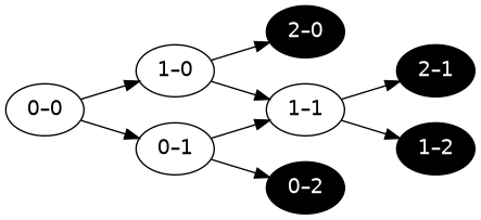
In the outcomes represented by the two top black nodes, we need to be in possession of $2, and in the bottom two nodes, nothing. For clarity, let’s add this information to the graph.
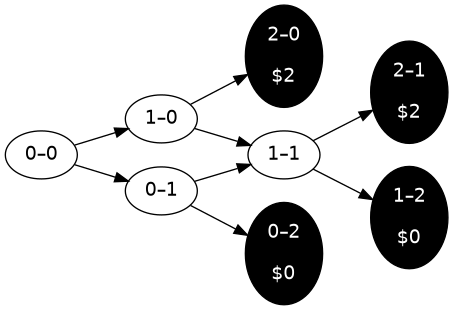
This puts a constraint on the 1–1 game: we need to place a bet such that if Alpha wins, we get $2, and if Alpha loses, we have nothing. Some thinking will lead to the answer: before that game, we must be in possession of $1, and place it all on Alpha winning the game. We’ll add that to the graph too.
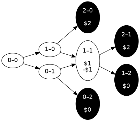
Now the process repeats. This has put a constraint on the 1–0 game. We have to possess and wager money such that if Alpha wins, we have $2, and if Alpha loses, we still have $1. This can only happen if we have $1.5, and wager $0.5. This continues all the way to the first game:
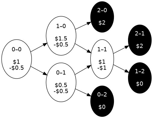
In other words, as long as the odds for all games are set in advance, we can replicate the 2:1 series bet by cleverly betting on the individual games. We figured out how by conditioning on the outcome of earlier games.
Spreadsheet Sketch
In this small number of games, we could do the calculations manually. If the teams play more games, we might want to make a spreadsheet. If we tilt our head, the nodes in the graphs above actually sort of make up a coordinate system, where each axis counts the number of wins by the corresponding team.
So we can start our spreadsheet by filling in the boundary conditions, here for a first-to-three-wins series, again, with 2:1 odds on both individual games and the series. In each cell is the amount of money we have in the outcome in question.
| 0 wins A | 1 win A | 2 wins A | 3 wins A | |
| 0 wins B | 2 | |||
| 1 win B | 2 | |||
| 2 wins B | 2 | |||
| 3 wins B | 0 | 0 | 0 | – |
Now, for each game, we have the following equations:
\[w + x = R\]
\[w - x = D\]
where \(w\) is wealth before the game, \(x\) is bet size, \(R\) is the cell to the right and \(D\) is the cell below. We can add those together to cancel out the bet size, and then we learn that
\[2w = R + D\]
or simply that the wealth in each cell should be the average of the win and the loss on that bet. (Due to the 2:1 odds.)
We plug this in and autofill from the bottom right to the top left.
| 0 wins A | 1 win A | 2 wins A | 3 wins A | |
| 0 wins B | 1.00 | 1.38 | 1.75 | 2 |
| 1 win B | 0.63 | 1.00 | 1.50 | 2 |
| 2 wins B | 0.25 | 0.5 | 1.00 | 2 |
| 3 wins B | 0 | 0 | 0 | – |
This doesn’t tell us directly how to bet, only how much money to have in various situations. But we can derive how much to bet from this, using the same equations as above.
If the odds are something other than 2:1, e.g. 1.63, we would end up with only a tiny bit more complicated equations:
\[w + 0.63x = R\]
\[w - x = D\]
which combined give us \(w = (1.59R + W)/2.59\). If we plug that formula into our spreadsheet instead, we’ll see that to end up with $1 if A wins, we have to start with $0.71.
| 0 wins A | 1 win A | 2 wins A | 3 wins A | |
| 0 wins B | 0.71 | 0.83 | 0.94 | 1 |
| 1 win B | 0.50 | 0.67 | 0.85 | 1 |
| 2 wins B | 0.23 | 0.38 | 0.61 | 1 |
| 3 wins B | 0 | 0 | 0 | – |
From this, we learn that the appropriate odds for the entire series, based on the odds for the individual games, is 0.71:1, or 1.41 decimal.
Reflection On Probabilities
Isn’t that last result interesting? When the there’s 1.63 odds on Alpha in the individual games, the odds on Alpha taking the entire series is 1.41!
It becomes less confusing if we look at it through the lens of probability. The odds imply a win probability of 61 % on the individual games, but just over 70 % on the series. This is but an application of the central limit theorem: winning the series is sort of like flipping more heads than tails when tossing a biased coin. As long as the bias is positive, even if it is small, flip enough times and we’re almost guaranteed to have more heads than tails.12 One could write an entire article on different ways to look at this situation, but I’m not going to for now!
But look how we got there! We didn’t touch probabilities once in our evaluations of odds, we just reasoned based on how our wealth is transformed from wagering, and we ended up sorta-kinda loosely confirming a common law of probability.